The following examples of current research give a flavor of the types of science studies that are currently underway. The scientific goals are to better understand the distribution and propagation of atmospheric waves and their effects on the ionosphere, thermosphere, and mesosphere (ITM).
Data Assimilation in the Mesosphere and Lower Thermosphere
Movie Caption: Animations of the meridional wind at the surface (bottom panel) and near 100 km (top panel). Key Points: Wave features and the background flow evolve much more rapidly at 100 km than at the surface. These different time-scales demand different data assimilation methods in the mesosphere-thermosphere-ionosphere (MTI) compared to in the troposphere.
The large-scale flow in the middle and upper atmosphere significantly influences the propagation of small-scale waves into the MTI. Data assimilation combines observations with a physics-based numerical model in order to provide the best estimate of the atmospheric state. It has been demonstrated that data assimilation significantly improves the representation of the large-scale dynamics of the middle atmosphere. This is despite the fact that existing whole atmosphere data assimilation systems have largely adopted techniques developed for numerical weather prediction, and are not yet tailored to the unique features of the MTI. These features include: drastically different temporal and spatial scales in the MTI compared to the troposphere-stratosphere; importance of preserving small-scale waves in the MTI; limited observing system in the MTI; and the difficulty in generating model ensembles due to external forcing of the MTI. During Phase 2 the WAVE team will improve data assimilation methods in the MTI.
Assessing the impact of middle atmosphere observations on day-to-day variability in lower thermospheric winds using WACCM-X
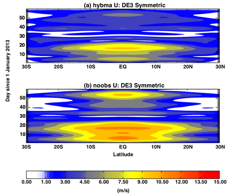
Figure Caption: At 100 km, the symmetric component of the nonmigrating DE3 tide in a simulation with middle atmosphere observations (hybma; a) and a simulation without middle atmosphere observations (noobs; b), as a function of latitude and time. Key Point: DE3 amplitude at 100 km is sensitive to middle atmosphere observations.
Recent studies have shown that day-to-day variability in thermospheric winds (100–300 km altitude) driven by meteorological variability from below affects ionospheric E and lower F regions, highlighting the need for accurate, continuous specification of day-to-day variability throughout the entire atmosphere for geospace weather prediction systems. To better understand the nature of forcing from below on the coupled thermosphere/ionosphere system, this study uses the Specified Dynamics Whole Atmosphere Community Climate Model eXtended (SD-WACCM-X) to quantify how the meteorology of the underlying atmosphere impacts the thermosphere. Global meteorological specifications are produced by a high-altitude version of the Navy Global Environmental Model (NAVGEM-HA), which assimilates standard meteorological observations from the surface through the lower atmosphere, and satellite-based observations of temperature and constituents in the middle atmosphere (MA) from 10–90 km altitude. Two SD-WACCM-X simulations for the January–February 2013 period are performed using NAVGEM-HA specifications produced with and without assimilation of MA observations. Results show that the availability of MA observations strongly constrains the modeled spectrum of planetary scale waves (zonal wavenumbers 1–3) in the thermosphere. Specifically, the amplitudes of the solar nonmigrating DE3 tide and westward quasi-two-day wave (Q2DW) are nearly twice as large in SD-WACCM-X simulations without MA observations compared to simulations with MA observations. Model diagnostics show that these differences are related to nonlinear wave-wave interactions impacting the DE3 mode and to sources of baroclinic/barotropic instability near the summer mesospheric easterly jet impacting the Q2DW. This study highlights the importance of MA observations for constraining whole atmosphere models needed for next generation space weather prediction capabilities.
Volcanic Eruptive Gravity Waves Over the Caribbean on 11 April 2021
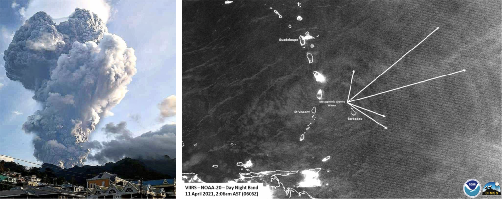
La Soufrière on Saint Vincent island in the Caribbean erupted explosively on 9-15 April 2021. Periods of banded tremors associated with explosive activity lasted for 20-30 minutes, with 1-3 hour gaps. The resulting ash plumes sometimes rose to 20 km altitude, “overshooting” the tropopause and exciting gravity waves that propagated into the upper atmosphere. These waves caused ripple patterns in the nightglow around 85 km altitude, which were observed in the NOAA satellite “Day Night Band” measurements, as shown by the white arrows in the right panel. Similar concentric ionosphere disturbances were also measured by GNSS (global navigation satellite system) instruments. This event is a compelling example of lithosphere-atmosphere-ionosphere coupling.
High Resolution Gravity Wave Modeling
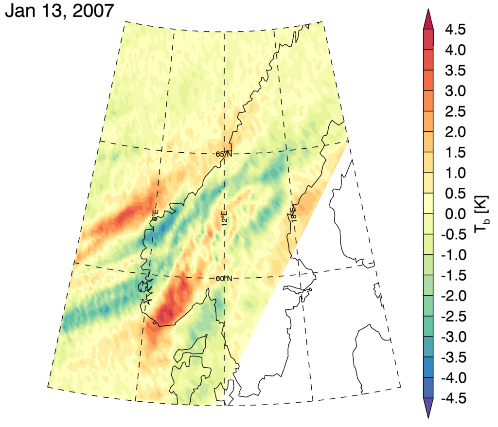
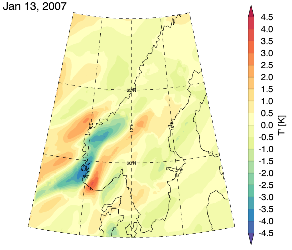
This figure shows a direct comparison of gravity wave brightness temperature anomalies observed by AIRS, the Atmospheric Infrared Sounder on NASA’s Aqua satellite (left panel) with those simulated in a high-resolution GEOS simulation, Geostationary Operational Environmental Satellite Program (right panel) in which the large-scale winds were constrained to reanalysis winds. The gravity waves in GEOS in this case are internally generated by model wind interactions with topography. The simulated gravity wave pattern and amplitude are remarkably realistic compared to the observed gravity wave characteristics, even though there is some fine-scale structure in AIRS that is not captured by the model. The realism of the simulated waves and the 3D regular output of the model provide an excellent opportunity to calculate the global distributions of the vector momentum flux, the associated gravity wave drag, and the sources of the gravity waves.
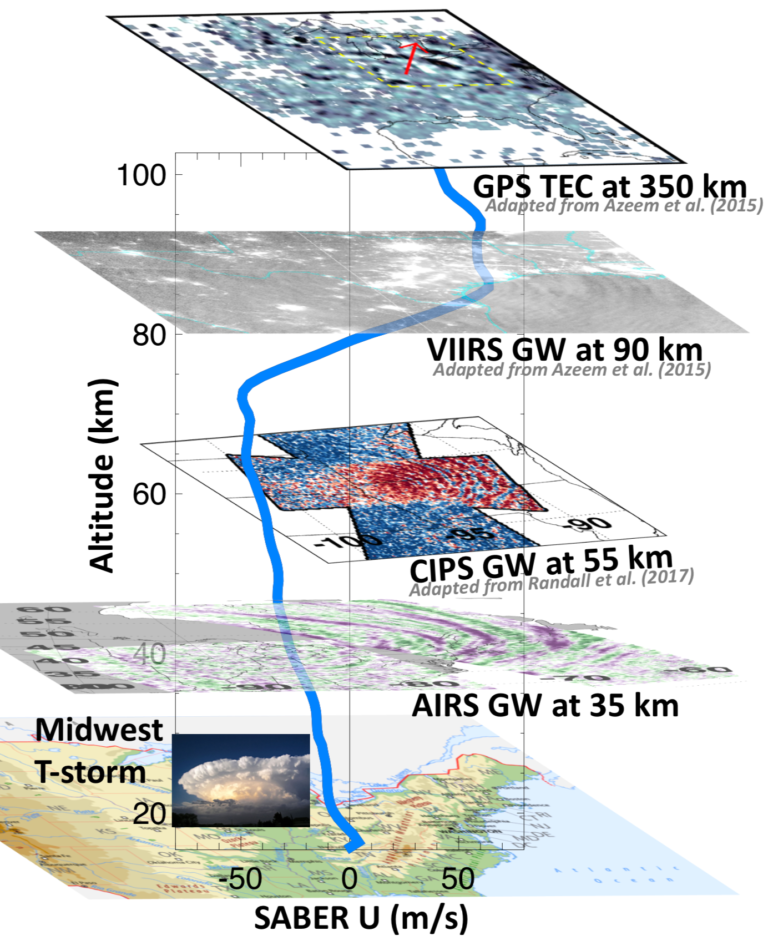
Combining Multiple Observational Platforms
The WAVE team makes use of the powerful technique of combining observations from multiple satellite platforms to trace gravity waves propagating from the lower atmosphere to the thermosphere and ionosphere. This is like taking CT Scans: Imaging gravity waves simultaneously at different atmospheric layers and studying the vertical evolution of gravity waves. In this way, the gravity wave-induced impact on space weather can be accurately traced back to its lower altitude source. Some gravity waves break in the middle atmosphere and excite higher order gravity waves. By combining observations of gravity waves at a variety of altitudes one can see both the primary waves and the higher order waves responsible for ionospheric variability. This approach leverages many relevant NASA Heliophysics and Earth Science satellite assets and maximizes their scientific return.
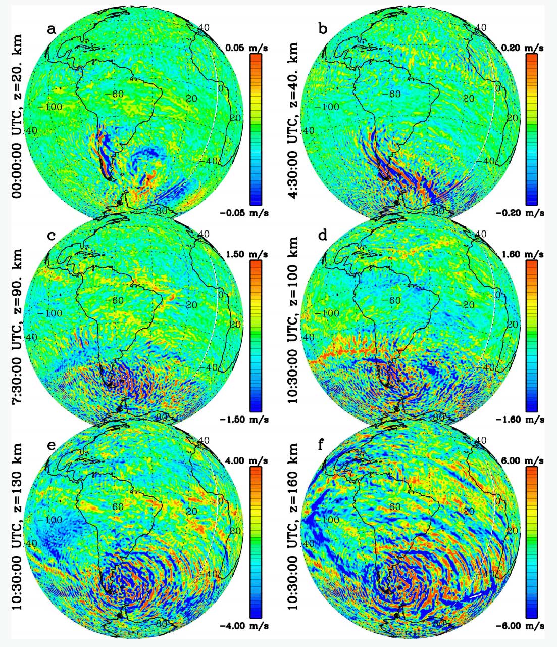
Modeling Gravity Waves through the Whole Atmosphere
This figure shows the vertical velocity at altitudes of 20 to 160 km from the free-running KMCM model during a mountain wave event over the Southern Andes. During this event, strong winds blow over the Southern Andes and excite mountain waves. These mountain waves, which are atmospheric gravity waves (GWs), propagate well into the stratosphere because of the strong polar night jet, which enhances vertical propagation of mountain waves (upper row). The mountain waves break and dissipate at altitudes of 50-70 km, which results in the deposition of energy and momentum there. These sources create secondary GWs which propagate up into the mesosphere and lower thermosphere region (middle row). These secondary GWs then break and dissipate, which via the same process, excite tertiary GWs that propagate well into the thermosphere (circular rings in the lower panel). See Vadas & Becker (2019) for more details. This study is important because it shows that energy from below (in this case, wind blowing over mountains) can be transferred to wave energy in the upper atmosphere via this multi-step vertical coupling process. Thus accurate modeling of waves in the F region of the ionosphere needs to take into account wave sources from below. Current state-of-the-art whole atmosphere models with GW parameterizations do not account for higher-order wave influences. This is aprime motivation for the WAVE science center.Vadas, S.L. & E. Becker (2019), Numerical Modeling of the Generation of Tertiary Gravity Waves in the Mesosphere and Thermosphere During Strong Mountain Wave Events Over the Southern Andes, J. Geophys. Res. Space Physics, https://doi.org/10.1029/2019JA026694
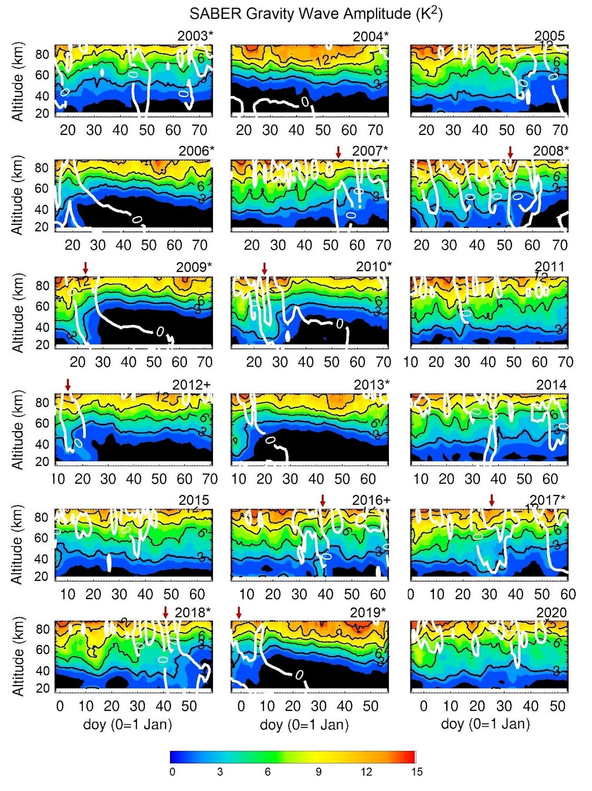
Gravity Wave Temperature Amplitude from 18 years of SABER Observations
Figure caption: Zonal mean gravity wave (GW) amplitude (K2) averaged over 60-85°N for 18 years of SABER observations. The zero wind (zonal mean zonal gradient wind derived from SABER geopotential) line is shown as white contours. The arrows on the top x-axis indicate the first day of wind reversal at 30 km during stratospheric sudden warming (SSW) events (* = major warming year, + = minor warming year).
GW amplitudes grow with increasing altitude due to the decrease in atmospheric density, i.e., the effect of energy density conservation. In the stratosphere, the suppression of GW amplitude is observed after a SSW onset. Models show that the wind reversal from eastward to westward during SSW events suppresses orographic and westward propagating non-orographic GWs (SABER GW amplitudes do not provide wave propagation direction). A brief increase in GW amplitude is also observed before some SSW events (e.g., between day of year [doy] 20-30 and 25-40 km for years 2009 and 2010).
Fine-scale Shear Leads to Radiated Gravity Waves
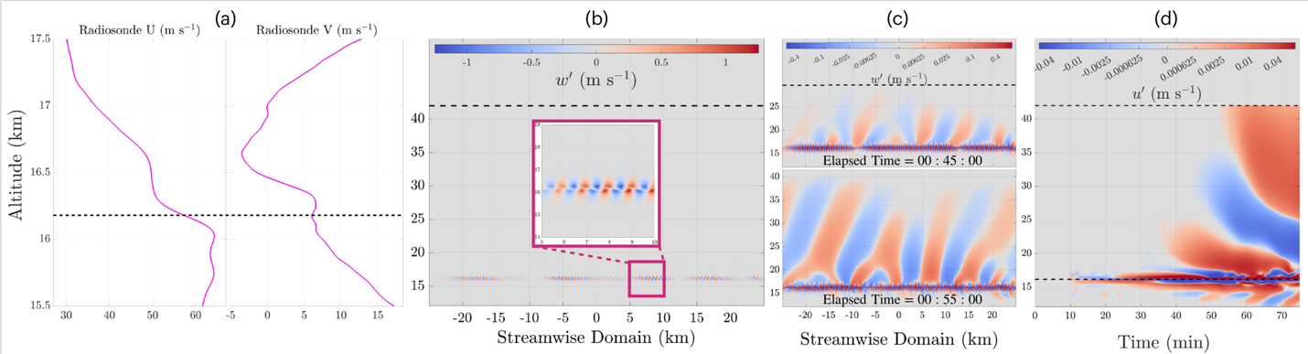
Figure Caption: (a) background wind profiles; (b) initial KHI formation in w’ field; (c) w’ radiated wave responses at 45 and 55 min elapsed times; (d) u’ altitude-time plot showing fishbone structure of radiated waves.
Non-orographic gravity wave sources occur in regions where breaking gravity waves and mesoscale jet/fronts generate instabilities that yield a resulting body force (e.g., Vadas et al. 2018). Fine-scale sheet and layer structures are an additional instability source produced by superposed local and large scale shear features that elevates local stratification throughout the atmosphere (Fritts et al., 2017 and citations therein). An investigation was undertaken to determine if these local instability sources can also produce radiated gravity waves in the stratosphere. Such wave sources could explain small-scale waves observed in airglow measurements (e.g., Medeiros et al., 2003; Nielsen et al., 2006) where propagation from the ground is unlikely.
Numerical simulations with the Complex Geometry Compressible Atmosphere Model (CGCAM, see e.g., Dong et al., 2021; Fritts et al., 2021) were initialized with the radiosonde wind profiles shown below in Figure 1a. These wind profiles show a clear superposition of a larger scale, ~3 km initial gravity wave and a localized ‘kink’ in the IGW phase that enhances the shear above. The combination of these shear sources produces a 100 m shear layer with a minimum Richardson number of 0.11 immediately below the layer.
3D Simulations were conducted in a deep domain with 50/30 km streamwise/vertical extents and a 500 m spanwise extent. The flow was seeded with small-amplitude, random noise fields in velocity and allowed to evolve with time. After 30 minutes elapsed time, KHI began to form at the layer (Figure 1b). At later times, radiated wave responses extend away from the shear layer with horizontal scales 5-10x larger than the initial KHI (Figure 1c). Altitude-time plots (Figure 1d) show a “fishbone” structure with downward (upward) phase propagation above (below) the layer, suggesting wave radiation consistent with the body force mechanism shown by Vadas et al., 2018 at larger scales.
This investigation demonstrates that small-scale, local instability sources can radiate high frequency gravity waves in the stratosphere. Shear superpositions like these can occur ubiquitously throughout the atmosphere and may account for small-scales waves seen at higher altitudes. These dynamics occur at small spatial scales that cannot be resolved by general circulation models – we hope that investigations like this one can provide guidance for future model development to more accurately reflect wave dynamics in the real atmosphere.
References:
Dong, W., Fritts, D. C., Thomas, G. E., & Lund, T. S. (2021). Modeling responses of polar mesospheric clouds to gravity wave and instability dynamics and induced large-scale motions. Journal of Geophysical Research: Atmospheres, 126, e2021JD034643. https://doi.org/10.1029/2021JD034643
Fritts, D. C., Wang, L., Baumgarten, G., Miller, A. D., Geller, M. A., Jones, G., Limon, M., Chapman, D., Didier, J., Kjellstrand, C. B., Araujo, D., Hillbrand, S., Korotkov, A., Tucker, G., & Vinokurov, J. (2017). High-Resolution Observations and Modeling of Turbulence Sources, Structures, and Intensities in the Upper Mesosphere. Journal of Atmospheric and Solar-Terrestrial Physics, November 2016, 1–22. https://doi.org/10.1016/j.jastp.2016.11.006
Fritts, D. C., Wieland, S. A., Lund, T. S., Thorpe, S. A., & Hecht, J. H. (2021). Kelvin‐Helmholtz billow interactions and instabilities in the mesosphere over the Andes Lidar Observatory: 2. Modeling and interpretation. Journal of Geophysical Research: Atmospheres, 126, e2020JD033412. https://doi.org/10.1029/2020JD033412
Medeiros, A. F., Taylor, M. J., Takahashi, H., Batista, P. P., & Gobbi, D. (2003). An investigation of gravity wave activity in the low‐latitude upper mesosphere: Propagation direction and wind filtering. Journal of Geophysical Research, 108(D14) , 4411. https://doi.org/10.1029/2002JD002593
Nielsen, K., Taylor, M. J., Stockwell, R. G., & Jarvis, M. J. (2006). An unusual mesospheric bore event observed at high latitudes over Antarctica. Geophysical Research Letters ,33, L07803. https://doi.org/10.1029/2005GL025649
Vadas, S. L., Zhao, J., Chu, X., & Becker, E. (2018). The excitation of secondary gravity waves from local body forces: Theory and observation. Journal of Geophysical Research: Atmospheres, 123, 9296–9325. https://doi.org/10.1029/2017JD027970
Sampling Strategies for Training Machine Learning Emulators of Gravity Wave Parameterizations
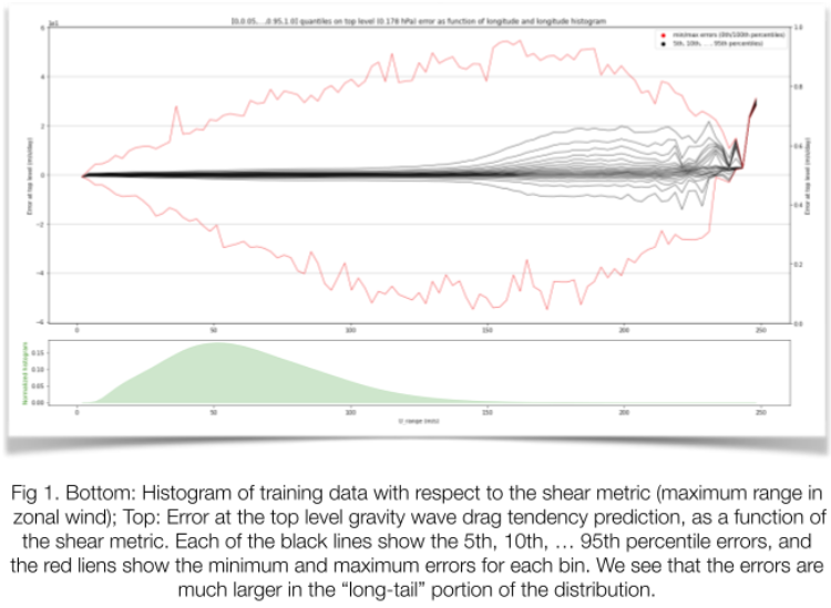
With the ultimate goal of developing a data-driven parameterization of gravity waves (GWs) for use in general circulation models (GCMs), we investigate various machine learning (ML) architectures that emulate the Alexander-Dunkerton ’99 (AD99) scheme, an existing GW parameterization. We analyze the distribution of errors as functions of shear-related metrics in an effort to diagnose the disparity between online and offline performance of the trained emulators, and develop a sampling algorithm to treat biases.
It has been shown in similar previous efforts [Espinosa et al., 2022] that stellar offline performance does not necessarily guarantee adequate performance online and can even lead to instabilities. A thorough error analysis reveals that the majority of the samples are learned quickly whereas some stubborn samples remain poorly represented. We find that the more error-prone samples are those with wind profiles that have large shears– this is corroborated with physical intuition as large shears indicate many breaking levels and therefore parameterizing gravity waves for samples with large shear wind profiles is a more difficult, complex task. To remedy this, we develop a sampling strategy that performs a parameterized histogram equalization, which is a key concept borrowed from 1D optimal transport.
The sampling algorithm uses a linear mapping from the original histogram to the uniform histogram parameterized by 0 ≤ t ≤ 1 where t=0 recovers the original histogram and t=1 the uniform histogram. A given value t assigns each bin a new probability which we then use to sample from each bin. If the new probability is smaller than the original, then we invoke sampling without replacement. If the new probability is larger than the original, then we repeat all the samples in the bin up to some predetermined “maximum repeat” value. We optimize this sampling algorithm with respect to t, the maximum repeat value, and the number and distribution (uniform or not) of the histogram bins. The ideal combination of those parameters yields errors that are closer to a constant function of the shear metrics while maintaining high accuracy over the whole dataset. Although we study the performance of this algorithm in the context of training a gravity wave parameterization emulator, this strategy can be used for learning datasets with long tail distributions where the “rare” samples are associated with low accuracy. Instances of this type of datasets are prevalent in earth system dynamics: launching of gravity waves, and extreme events like hurricanes, heat waves are just a few examples.
References:
Alexander, M. J., & Dunkerton, T. J. (1999). A Spectral Parameterization of Mean-Flow Forcing due to Breaking Gravity Waves. Journal of the Atmospheric Sciences, 56(24), 4167–4182. https://doi.org/10.1175/1520-0469(1999)056<4167:ASPOMF>2.0.CO;2
Espinosa, Z. I., A. Sheshadri, G. R. Cain, E. P. Gerber, and K. J. DallaSanta, 2021: A Deep Learning Parameterization of Gravity Wave Drag Coupled to an Atmospheric Global Climate Model, Geophys. Res. Lett., accepted.
Machine Learning for Gravity Wave Parameterization: Regression Tree Ensemble Approaches
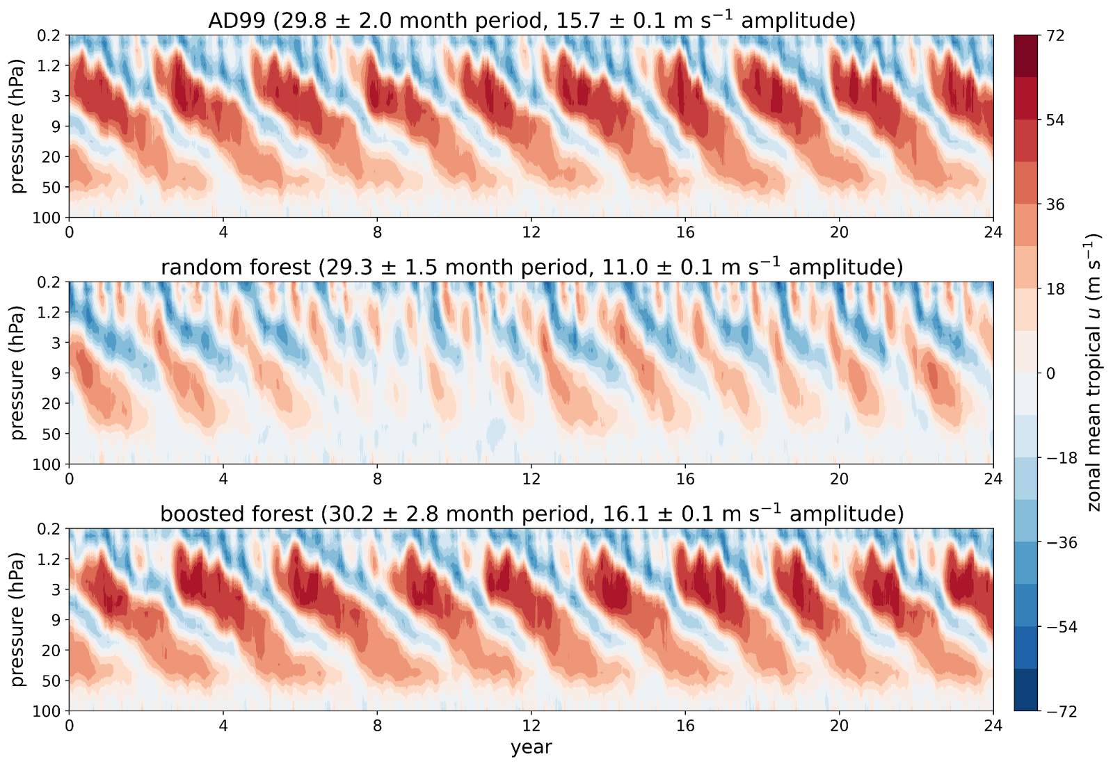
Figure Caption: Pressure-time sections of tropical zonal mean zonal wind in a model with different GW parameterizations: AD99 (top), random forest RTE (middle), and boosted forest RTE (bottom).
Gravity wave sources and length scales are often smaller than what can be resolved by global climate models (GCMs), and so their effects must be parameterized. Techniques from machine learning allow increasingly available observational datasets and high-resolution simulations to be used to develop data-driven parameterizations. As a first step, we train machine learning models to emulate the Alexander-Dunkerton 1999 (AD99) parameterization (Alexander & Dunkerton, 1999) in order to explore the performance of various methods. After a machine learning emulator is trained, it can be run online — that is, the GCM can be run using the gravity wave drag at each time step as calculated by the emulator instead of the original parameterization.
One indicator of climate realism for a gravity wave scheme is the Quasi-Biennial Oscillation (QBO), an alternating pattern of westerly and easterly winds in the tropical stratosphere. The figure shows the QBOs produced online by AD99 and two types of regression tree ensemble (RTE), a class of machine learning model, in MiMA, an intermediate-complexity GCM. The boosted forest emulator accurately reproduces the period and amplitude of the QBO from the original parameterization, while the random forest is less successful at driving a qualitatively correct QBO. Nonetheless, both emulators run stably when coupled with the GCM. This study demonstrates that RTEs can be powerful enough to emulate a gravity wave parameterization and seem to be naturally stable when run online. Further research will assess whether RTEs retain these qualities when trained on more realistic data sources.
References:
Alexander, M. J., & Dunkerton, T. J. (1999). A Spectral Parameterization of Mean-Flow Forcing due to Breaking Gravity Waves. Journal of the Atmospheric Sciences, 56(24), 4167–4182. https://doi.org/10.1175/1520-0469(1999)056<4167:ASPOMF>2.0.CO;2
Complex Wave Patterns in McMurdo Lidar Observations
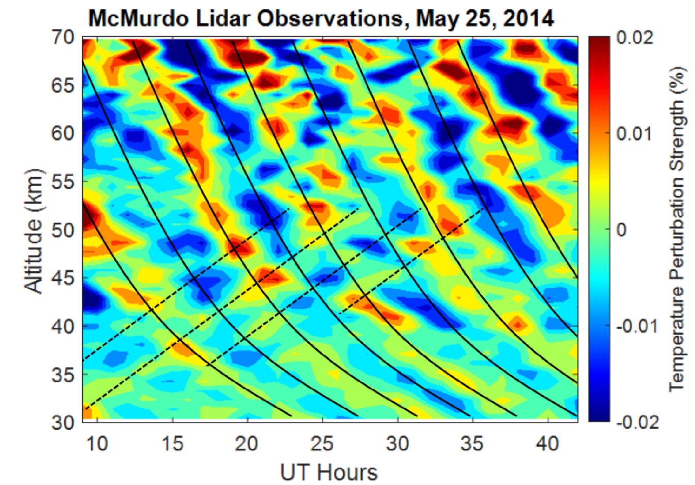
Figure Caption: Altitude-time section of lidar temperature perturbation strength observed at McMurdo station on 25 May 2014.
In this sample of relative temperature perturbations from a lidar observation taken via Rayleigh lidar at McMurdo, Antarctica, especially distinct and persistent waves can be seen throughout the entire observational window extending over 40 km in altitude and ~30 hrs in time. The reds show the warm phase of the wave, and the blues show the cold phase. These waves exhibit regular periods of ~8 hrs, though are not terdiurnal tides (Fong et al., 2014). Local phase speeds appear to exhibit a turn around 45 km.
Highlighted by the black solid lines are waves exhibiting downward phase-progression and in the black dashed lines are waves showing upwards phase-progression, forming a “checkerboard” pattern at the central altitudes of this observation. Wave patterns like this are not uncommon in Antarctic lidar observations and this sample highlights the power of observations in studying complex wave behavior and wave interactions in the middle and upper atmosphere.
For info about the McMurdo lidar campaign see:
http://cires1.colorado.edu/science/groups/chu/pubs/
Chu, Huang, et al., 2011. https://doi.org/10.1029/2011GL048373
Chu, Yu, et al., 2011. https://doi.org/10.1029/2011GL050016
Fong et al., 2014. https://doi.org/10.1002/2013JD020784
ICON Satellite Observations of Small-Scale Perturbations from 90 km to 250 km
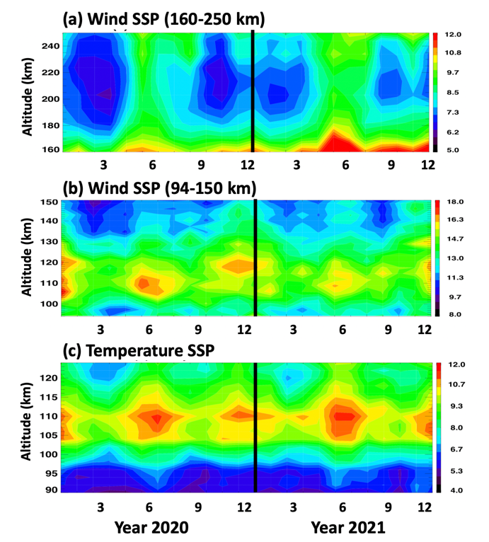
Figure Caption: Amplitudes of small-scale perturbations from MIGHTI (a, b) zonal winds and (c) temperature.
Gravity waves (GWs) from the troposphere to the thermosphere have an important role in atmospheric coupling processes. Due to observational difficulties, satellite measurements of GWs between the mesosphere and the lower thermosphere (MLT) region and the thermosphere (~250 km) are rare. The Ionospheric Connection Explorer (ICON) satellite was launched in 2019 and data has been available since December 2019. Here we use ICON MIGHTI (Michelson Interferometer for Global High-resolution Thermospheric Imaging) observations of zonal and meridional winds from 94 km to ~300 km and temperature from 90 km to 127 km (altitude coverage varies with local-time) to understand GW variations between 90 km to 250 km.
The figure above sshows gravity wave amplitudes from 94 km to 250 km measured by ICON-MIGHTI wind data. Gravity wave amplitudes show semi-annual variations with peaks in July-August and December-January below 150 km. Seasonal variations changes to annual variations above 160 km. Such changes coincident with when zonal wind reversal occur in December and January, which can affect GW propagation. GW observations from ~120 km to ~250 km are useful to validate high-resolution whole atmosphere models and understand roles and impacts of GWs on coupling processes.
Characterizing Persistent Gravity Waves in the Upper Atmosphere of Antarctica
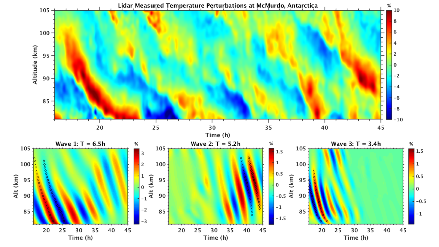
Figure Caption: Antarctica Altitude-time sections of temperature perturbations observed by a lidar at McMurdo Station, Antarctica (top). Decomposing wave-induced temperature perturbations measured by lidar into individual wave packets (bottom panels) using a 2D Morlet wavelet transform. This methodology is being used to characterize the intermittency and spectral properties of gravity waves in the upper atmosphere at McMurdo Station.
Strong and persistent gravity wave (GW) activity in the mesosphere and lower thermosphere (MLT) has been observed for 10+ years by lidar instruments deployed at McMurdo Station, Antarctica. The above figure demonstrates how an automated, 2D wavelet transform-based methodology is used to break a field of GW-induced temperature perturbations down into quasi-monochromatic wave packets, so that they may be studied individually. This sophisticated spectral analysis tool and 10 years of high-resolution lidar data are being used to statistically characterize the properties of the GWs in the upper atmosphere at McMurdo and investigate the variability associated with them. Vadas and Becker (2018) concluded from KMCM model results that the majority of these waves in the mesosphere and lower thermosphere are secondary GWs, rather than primary GWs originating from the troposphere. This observational study in progress has the potential to provide a reliable reference for the validation of GW-resolving models, as well as new insights into the multistep vertical coupling processes which transfer energy from the ground to ionospheric heights.
References:
Vadas, S. L., & Becker, E. (2018). Numerical modeling of the excitation, propagation, and dissipation of primary and secondary gravity waves during wintertime at McMurdo Station in the Antarctic. Journal of Geophysical Research: Atmospheres, 123, 9326-9369. https://doi.org/10.1029/2017JD027974