How to Load and Plot Data
DAXSS examples (Python)
Using a Graphical User Interface (GUI) based utility
Here is a link to the code. This utility provides a simple GUI for plotting and fitting DAXSS data. The user can select variables in the Level-1 file and plot parameters using the utility GUI, to create plots such as time-series plots and energy spectrum overlay plots. The utility also contains functionality to fit a particular spectra to standard models available in XSPEC (such as vvapec). The fit parameters such as energy range and elements to be fit can be selected using the menus in the utility GUI. The ReadMe page in the link shared above provides more instructions on installing dependencies and running the utility. For more information, contact Anant Kumar T K (anant.telikicherla@ualberta.ca).
Directly in Python
We’ve created a Google Colab notebook containing all of the code along with explanatory text so that you can follow along. The notebook provides code snippets for accessing DAXSS level-1 data, viewing variable metadata, creating spectra plots, and generating Pulse Height Analyzer (.PHA) files for spectral fitting using XSPEC (and PyXSPEC). These code snippets can be run directly in your browser, without the need for any dependency installation on your local machine. The tutorial also contains a code snippet for fitting DAXSS data to XSPEC models, that can be run on your local machine after installation of XSPEC and PyXSPEC. For more information, contact Anant Kumar T K (anant.telikicherla@ualberta.ca).
MinXSS examples (IDL and Python)
Loading data
First, simply download the mission-length level 1 MinXSS data (minxss1_l1_mission_length.sav). This link takes you to the file that is regenerated daily that folds in all new telemetry received.
IDLDE (IDL Workbench)
You can simply double click the minxss1_l1_mission_length.sav file and it will load the minxsslevel1 variable. You can alternatively load the data in the interactive console using the IDL console method below.
IDL console
restore, path + path_sep() + ‘minxss1_l1_mission_length_v2.sav’
where path is the path to the file. Also, make sure that filename is accurate in your case. The built-in path_sep() function is used above to return a / for Linux/Mac (i.e., Unix)
systems and a \ for Windows systems.
To see what variables are available inside the minxsslevel1 structure, just type:
help, minxsslevel1, /STRUCTURE
For each sub-structure there, you can follow the same pattern, e.g.,
help, minxsslevel1.x123, /STRUCTURE
Python (requires scipy)
from scipy.io.idl import readsav
data = readsav(‘path/minxss1_l1_mission_length_v2.sav’)
minxsslevel1 = data.minxsslevel1.x123[0].copy()
where path is the path to the file. This generates a dictionary (data) containing the variables minxsslevel1 and minxsslevel1meta. We copy minxsslevel1 out for convenience, so that you don’t have to call data.minxsslevel1 thereafter. minxsslevel1 is a numpy.recarray.
To see what variables are available inside the minxsslevel1 recarray, at an interactive prompt (e.g., IPython) type:
minxsslevel1.dtype.names
or if inside your script, just type the above inside of a print() statement.
Plotting data
1) A single spectrum
IDL
p = plot(minxsslevel1.x123[2913].energy, minxsslevel1.x123[2913].irradiance, $
TITLE = ‘MinXSS Solar SXR Spectrum on ‘ + $
minxsslevel1.x123[2913].time.human, $
XTITLE = ‘Energy [keV]’, XRANGE = [0.8, 2.5], $
YTITLE = ‘Irradiance [photons / sec / cm$^2$ / keV]’, YRANGE = [1e4, 1e9], $
/YLOG)
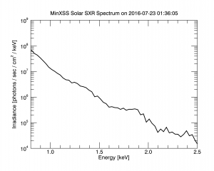
which should result in this plot:
An IDL procedure that loads the data and creates the above plot can be downloaded here.
Python
%matplotlib inline
import matplotlib.pyplot as plt
spectrum_index = 2913
plt.plot(minxsslevel1[spectrum_index][‘energy’], minxsslevel1[spectrum_index][‘irradiance’], drawstyle = ‘steps-mid’)
plt.xlim([0.8, 2.5])
plt.xlabel(‘Energy [keV]’)
plt.ylim([1e4, 1e9])
plt.yscale(‘log’)
plt.ylabel(‘Irradiance [photons / sec / cm$^2$ / keV]’)
plt.suptitle(‘MinXSS Solar SXR Spectrum on ‘ + minxsslevel1[spectrum_index][‘time’][‘human’][0].decode(“utf-8”))
plt.show()
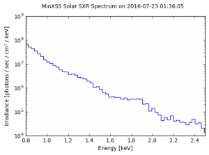
which should result in this plot:
A python notebook that loads the data and creates the above plot can be downloaded here.
2) A time series of a single bin
You would normally want to do this for an emission line. An emission line may cover multiple bins or multiple emission lines may fill an individual bin. For simplicity, we show you the principle here by plotting just a single bin corresponding to an energy of ~2 keV.
IDL
p1 = plot(minxsslevel1.x123.time.jd, minxsslevel1.x123.irradiance[73], $
SYMBOL = ‘dot‘, SYM_THICK = 3, COLOR = ‘dodger blue’, $
DIMENSIONS = [800, 600], $
TITLE = ‘MinXSS Solar SXR ‘ + $
strtrim(minxsslevel1.x123[0].energy[73], 2) + ‘ keV Over Time’, $
XTITLE = ‘Time [UTC]’, $
XTICKFORMAT = [‘LABEL_DATE’, ‘LABEL_DATE’], $
XTICKUNITS = [‘Month’, ‘Year’], $
XTICKINTERVAL = 1, $
YTITLE = ‘Irradiance [photons / sec / cm$^2$ / keV]’)
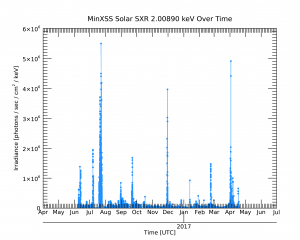
which should result in this plot:
An IDL procedure that loads the data and creates the above plot can be downloaded here.
Python
%matplotlib inline
from scipy.io.idl import readsav
import matplotlib.pyplot as plt
import numpy as np
import datetime
import matplotlib.dates as mdates
# Extract irradiance for the 73th bin corresponding to energy 2.0 keV
irradiance = minxsslevel1[‘irradiance’]
irradianceBin73 = np.zeros(len(irradiance))
for i in range(len(irradiance)):
irradianceBin73[i] = irradiance[i][73]
# Extract time and convert it so that matplotlib can understand it
time_human = []
for i in range(len(irradiance)):
time_human.append(minxsslevel1[i][‘time’][‘human’][0].decode(“utf-8”))
datetimes = [datetime.datetime.strptime(t, “%Y-%m-%d %H:%M:%S”) for t in time_human]
# Make the plot
fig, ax = plt.subplots(1)
plt.plot(datetimes, irradianceBin73, ‘b-o’, markersize = 3)
fig.autofmt_xdate()
ax.xaxis.set_major_formatter(mdates.DateFormatter(“%Y-%b-%d“))
plt.xlabel(‘Time [UTC]’)
plt.ylabel(‘Irradiance [photons / sec / cm$^2$ / keV]’)
plt.ylim([0, 8e8])
plt.suptitle(‘MinXSS Solar SXR ‘ + str(minxsslevel1[0][‘energy’][73]) + ‘ keV Over Time’)
plt.show()
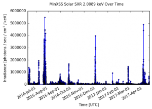
which should result in this plot:
A python notebook that loads the data and creates the above plot can be downloaded here.


